S4Explorer Structure Diagram: WHERE, JOIN and Associations

In Short

S4Explorer is a S/4 HANA Fiori app for exploring and analyzing S/4 HANA business content.

With S4Explorer, architects, consultants, developers and system administrators can quickly find and understand S/4 HANA objects like CDS views, table functions and OData Services. S4Explorer gives you quick and clear insights in how CDS objects work, how they support APIs and services, and visualize interconnections between all these aspects.

This series of blogposts highlights the main features of S4Explorer.

• The first installment of the series covered how Smart Search helps you to quickly find the CDS objects you’re interested in.
• In the second installment, we explained how CDS Structure Diagrams let you visually explore CDS objects, allowing you to grasp the design of even complex objects in just a glance by breaking down their structure in a layer of parameters (representing input), a data foundation (representing data transformation), and the projection list (representing output).

This third installment takes a further look at the CDS Structure Diagram, and explains how it visualizes features like JOINs, associations and WHERE-clauses.

Example 1: I_CarryForwardBudgetAccount

First, let’s take a look at theI_CarryForwardBudgetAccountCDS view. Here is its CDS source:

define view I_CarryForwardBudgetAccount as

select 
from        psm_d_glacctx as Main

inner join  ska1 
on          ska1.ktopl    = Main.chrt_accts
and         ska1.saknr    = Main.gl_account

association [0..1] to I_ChartOfAccounts as _ChartOfAccounts 
on          $projection.ChartOfAccounts = _ChartOfAccounts.ChartOfAccounts

association [0..*] to I_BudgetAccountText as _Text 
on          $projection.ChartOfAccounts = _Text.ChartOfAccounts
and         $projection.PubSecBdgtAcctCarryFwdTo = _Text.PubSecBudgetAccount

{
key cast( Main.chrt_accts as fis_ktopl preserving type )           as ChartOfAccounts,
key cast( Main.gl_account as psm_bdgt_acct_cf_to preserving type ) as PubSecBdgtAcctCarryFwdTo,
    cast( ska1.sakan as psm_bdgt_acct_cf_ext preserving type )     as PubSecBdgtAcctCarryFwdExt,
    _ChartOfAccounts,
    _Text
}

where      Main.bdgt_acct_rev_or_exp <> ''
and        Main.bdgt_acct_cf_use      = 'X'

This is how S4Explorer visualizes the view in the Structure Diagram:

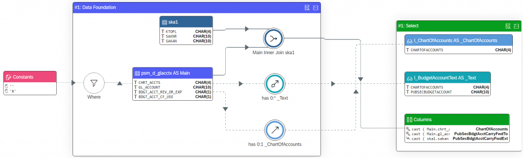
If you haven’t read the Structrure Diagram Primer yet (the previous installment in this series), you may want to take a few minutes to do that first. It introduces a bit of terminology that we rely on in this post as well.

JOIN-Operations

In the Structure Diagram Primer we saw a couple examples of CDS structure diagrams, but they would always have only a single data source node in the data foundation. The I_CarryForwardBudgetAccountCDS view contains an INNER JOIN between base tables psm_d_glacctx and ska1:

from        psm_d_glacctx as Main

inner join  ska1 
on          ska1.ktopl    = Main.chrt_accts
and         ska1.saknr    = Main.gl_account

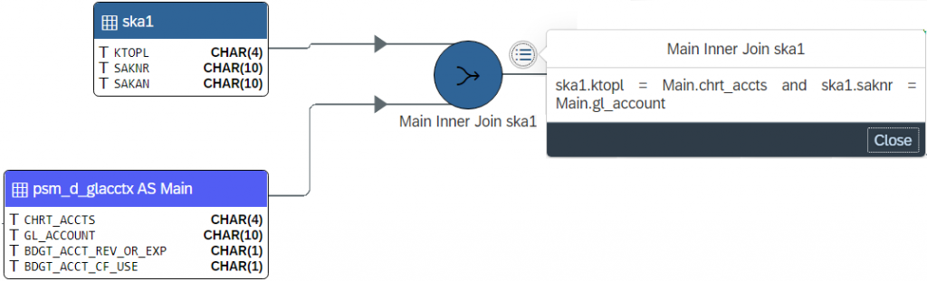
In the Structure Diagram, joins operations are represented by a circular node with a fiori Combine icon. The join node has a label identifying the datasources as well as the join type (INNER, LEFT OUTER, etc). The verbosity of the join label can be controlled from the settings panel (on the right of the structure diagram). The example shown here demonstrates the “full” join title, whereas a “short” title would only indicate the join type.

You can click on the join node and then press its detail action button. This reveals the CDS code that makes up the join condition used to combine the rows from the two datasources.

Joined data sources have outgoing lines pointing into the join node, indicating that their data flows into the join operator. In the example, these are solid lines, because this is an INNER JOIN. In case of a (LEFT or RIGHT) OUTER JOIN, the “outer”-joined datasource would lead a dashed line into the join node. The dashed line indicates that that datasource optionally yields rows matching the join condition.

The (conceptual) result of the join operation is represented by a line coming out of the join node. In the example, the outgoing line is lead into the Columns node in the Select group, but in more complex views, with more than one join, this line would be one of the inputs of the next join node.

You may notice that the two datasources each have a different header color. The first datasource that appears in the view (in this case: psm_d_glacctx) has a bright blue header. The second datasource (ska1) has a header of a darker shade of blue.

You can think of  psm_d_glacctx as the “leading” table and the conceptual point of departure in the data flow. From there, you follow its outgoing line throughout the data foundation, leading you along a single path, visiting all joined data sources.

With respect to the datasources, you may notice that the icon in this example is different from the ones we saw in the Structure Diagram Primer. In this case, the datasources are both base tables, and this is expressed by the fiori table-view icon.

In the example, the titles of the datasources are in long format, showing both the name of the data source (in this case, the base table name) and the alias (if present). You can control the verbosity of the data source titles from the settings panel, just like you can for the titles of the join nodes.

Hierarchical vs Sequential Join styles

In the example, the join node combines the main data flow with the joined data source. The join node then proceeds into its own outgoing data flow. This visual representation closely matches the conceptual operation of a join, yielding a new tabular result that combines rows from both its datasources.

Some CDS objects may benefit from a more simplified layout, representing the join as a straight flow from one datasource to the next. The settings panel lets you choose the layout. The default layout is hierarchical, and the simplifield layout is called sequential. The following screenshot illustrates the sequential join layout:

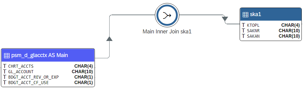
The sequential layout offers a clearer data flow, which is especiallly useful for complex CDS views with many JOINs. The disadvantage is that it contradicts what really happens in a JOIN operation. The JOIN refers to both the data source on its left and on its right side. At the same time, the data flow arrows suggest that the right table is reached after the JOIN.

S4Explorer lets you choose which layout you prefer. It doesn’t change the structure of the view – it’s just a matter of how you prefer to visualize it.

Constants and WHERE-Clause

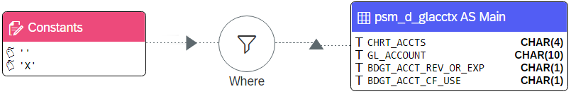
The example view has a WHERE-clause that restricts which rows are selected from the psm_d_glacctx datasource based on a few literal string values:

where      Main.bdgt_acct_rev_or_exp <> ''
and        Main.bdgt_acct_cf_use      = 'X'

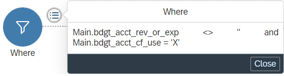
In the diagram, the WHERE-clause is represented by a circular node with a Fiori filter icon:

Just like with the join node, you can click the WHERE-clause node and press its details action button to reveal the CDS code that makes up the condition:

The lines coming into the WHERE-clause node from the constants node and the datasource represent the expressions that are combined inside the WHERE-clause.

You may be surprised to see the node representing the WHERE-clause out of line with the data flow going from data source to data source via the join nodes. If so then that’s probably because you think of the example view as taking data from the psm_d_glacctx datasource, then applying the condition in the WHERE-clause and leading the filtered dataset into the join operation (and so on).

However, there are many cases that won’t fit such a dataflow. A CDS view can only have one WHERE-clause, which may reference any data source appearing in the CDS view – independent from any JOINs. So conceptually, it’s the other way around: first, datasources are joined, and then the resulting dataset is filtered by the WHERE-clause.

No matter how you think of it, the point is that the CDS Structure Diagram makes it easy for you to spot the WHERE-clause and lets you see at a glance which columns, parameters and constants it uses.

Associations

S4Explorer distinguishes associations according to their type:

• Associations
• Compositions

In addition, S4Explorer distinguishes associations according to their maximum cardinality:

• maximum cardinality of 1: true associations
• maximum cardinality larger than 1: aggregations

In Object-oriented contexts, relationships between objects with maximum cardinality 1 are called associations. Those with maximum cardinality exceeding 1 are called aggregations.
The reason for this distinction is that aggregations affect the granularity of resultset and thus require special handling in applications. For this reason, S4Explorer visualizes them differently as well.

Associations with max cardinality of 1: True Associations

In the exmple, the first association is a 0..1 association called _ChartOfAccounts to I_ChartOfAccounts:

association [0..1] to I_ChartOfAccounts as _ChartOfAccounts 
on          $projection.ChartOfAccounts = _ChartOfAccounts.ChartOfAccounts

The structure diagram represents association definitions using a circular node. The node has a label with the name of the association, and also includes the association’s cardinality. The Fiori association icon and the light blue color also indicate the maximum cardinality of 1:

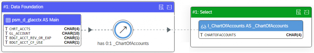
The association node has an outgoing line that points into the associated data source, in this case: I_ChartOfAccounts. This line is dashed, indicating that the relationship is optional, in accordance with the minimum cardinality of 0.

In the example, the _ChartOfAccounts association is exposed in the view’s SELECT-list. This allows other views that would select from this view to access the associated datasource. The structure diagram places such associated datasources in the SELECT-group to indicate that they are exposed and selectable.

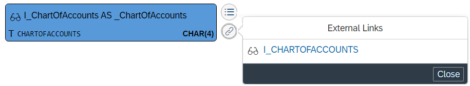
The associated datasource is itself a CDS view. That means we can select it, and use the links action button to navigate directly to it:

The line coming from datasource psm_d_glacctx into the association node represents the fact that the condition upon which the association is defined, references columns from that datasource. This may not be immediately clear when we look at the CDS code that defines the association’s ON condition:

on $projection.ChartOfAccounts = _ChartOfAccounts.ChartOfAccounts

Howevever, the expression $projection.ChartOfAccounts references another expression from the select list, which is defined as:

key cast( Main.chrt_accts as fis_ktopl preserving type )           as ChartOfAccounts

From that definition we can see that $projection.ChartOfAccounts is really a cast operation on the chrt_accts column from the psm_d_glacctx datasource. The line coming into the association node represents that relationship.

This type of pattern, where ON conditions for associations are defined based on $projection expressions is ubiquitous. By breaking down these CDS expressions, S4Explorer makes it a lot easier to see the actual relationships between datasources.

Of course, if you just want to see the bare CDS code of association’s ON condition, you can simply select the association node and press its detail action button to reveal it:

Associations with max cardinality > 1: Aggregations

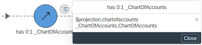
The second associations is a 0..* association called _Text to I_BudgetAccountText:

association [0..*] to I_BudgetAccountText as _Text 
on          $projection.ChartOfAccounts = _Text.ChartOfAccounts
and         $projection.PubSecBdgtAcctCarryFwdTo = _Text.PubSecBudgetAccount

This is how its visualized in the CDS structure diagram:

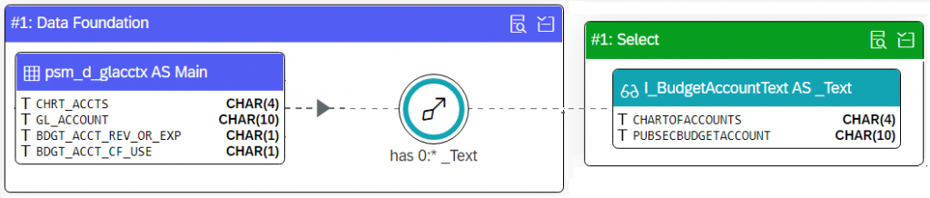
The feature and presentation are similar to what we just discussed for the _ChartOfAccounts association. The main difference is that the aggregation uses the Fiori aggregation icon and a sea-greenish color.

More CDS Structure, and beyond

In previous installment, we covered only a very simply view as a primer into S4Explorer Structure Diagrams. In this post, we covered a slightly more advanced view with JOINs, a WHERE-clause, and two different kinds of associations. There’s a few more structural elements we haven’t covered yet – GROUP BY, UNION and view extensions. We’ll cover those in a next installment of our S4Explorer feature highlights.

Finally

I hope this post helped you to understand a little bit more about S4Explorer’s CDS Structure Diagram. If you want to learn more about S4Explorer, then consider these resources:

• S4Explorer Smart Search – the first installmant in the S4Explorer feature hightlights series.
• S4Explorer Structure Diagram Primer – the second installment in the S4Explorer feature hightlights series and an introduction to S4Explorer Structure Diagrams.
• S4Explorer Product Page – learn about the features, pricing, or schedule an appointment for a live demo;
• Youtube video of our SAP Tech Talk: “S4Explorer – A Clear View Into S/4 HANA”, hosted by Product Manager Gabriel Garcia Mayorca;