Virtual Insanity
In 1996, the artist Jamiroquai released the song Virtual Insanity. In that song he predicts a future where we as a people are threatened by technology. Trying to figure out how SAP BW’s relatively new virtual InfoProviders work might drive one virtually insane. To prevent any BW modelers from experiencing virtual insanity, I’ve penned 2 articles about BW’s Virtual InfoProviders. This article is about the HANA CompositeProvider (HCPR). You can check out Part I, which covers the Open ODS View, here. In this article, I’m going to show you how to create a CompositeProvider and model it.
Here’s an overview of the topics discussed in Part II of this article. You can click a topic to jump to that particular section:
- Modeling Joins & Unions
- Creating Assignments
- Creating a Join Condition
- Adding joined fields to the Target
Why use a HANA CompositeProvider, and how?
Let’s assume you’ve modelled an Open ODS View. Now let’s say you want to do a Join or a Union between that data and another InfoProvider. This is where the CompositeProvider comes in. There are three different types of CompositeProviders:
- Ad hoc CompositeProviders, which can contain InfoProviders and Analytic Indexes and are created in the Data Warehousing Workbench or Analysis Process Designer.
- Local CompositeProviders, which you access via BW Workspace Designer and can contain local data.
- Central CompositeProviders, which can contain InfoProviders and SAP HANA Views. Central CompositeProviders replace ad hoc CompositeProviders if you use SAP HANA.
In this article, we’re only going to discuss number 3: The Central CompositeProviders, which we use in Eclipse and HANA.
Adding PartProviders
First, we’re going to add all the InfoProviders we want to use in this CompositeProvider. Right-click a folder in Eclipse in BW on HANA. Or right-click the Data Flow Modeler if you’re new school and are modelling in BW/4HANA. After you select CompositeProvider, you see the following screen:
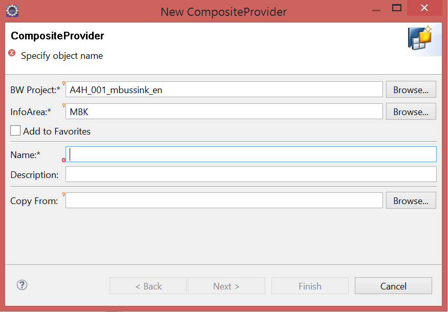
Figure 1. New CompositeProvider
After you fill in the straightforward stuff, like name and description, you get to the following screen:
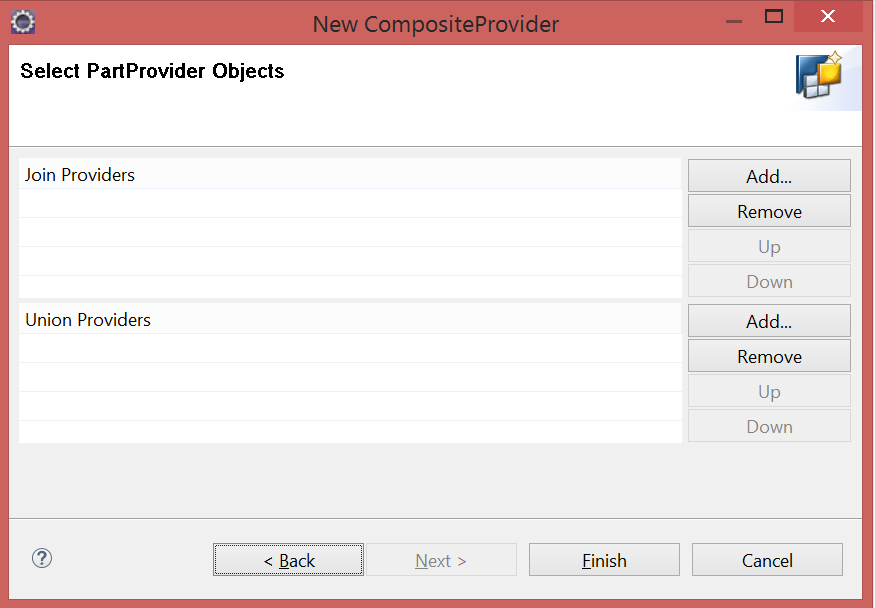
Figure 2. Select PartProvider Objects
In this screen, you select all the InfoProviders/PartProviders you want to Join or Union. If you change your mind after this step, no worries, because you can add and remove PartProviders later in the CompositeProvider modeling screen. In Figure 3 we see the PartProviders we can select when we press Add:
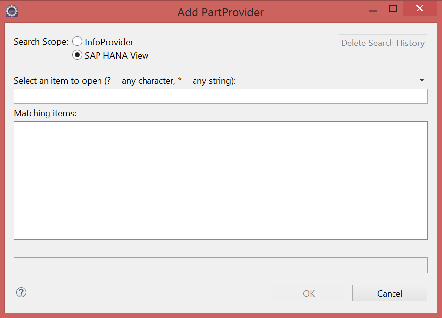
Figure 3. Add PartProvider screen
Here we see something interesting. Not only can we use InfoProviders in our CompositeProvider, we can also use SAP HANA Views. HANA developers rejoice! I won’t go further in-depth on the topic of using HANA Views in a HCPR. Reason being, HANA Views are modeled the same as field-based InfoProviders, which we use in this article. However, if you want to use HANA Views in a HCPR, you’ll first have to attach the SAP HANA System that contains those HANA Views to your BW Project.
Modeling in the Scenario Tab
After you press Finish in the screen after Figure 3, you’ll now be able to do the fun activity of modeling your CompositeProvider Joins & Unions. In the General Tab you can find query runtime settings, such as parallel processing, caching and the query read mode. The modeling happens in the Scenario Tab (see Figure 4).
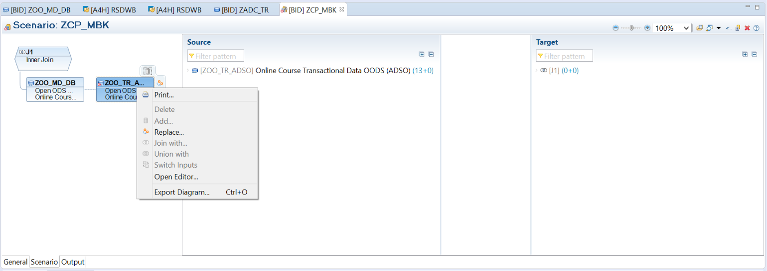
Figure 4. The Scenario Tab
In Figure 4 we see that the screen is split up into 3 segments:
- The left part of the screen where we indicate whether we want to use a Join and/or Union
- The Source area
- The Target area
Modeling Joins & Unions
Let’s start off by discussing the section on the left (see Figure 5). This section is where we indicate which InfoProviders we want to add additionally (in case of a Union) and delete. We can also replace the PartProviders we chose in an earlier screen if we’ve changed our mind. Because the CompositeProvider is a virtual object, we can change source objects with relative ease by selecting Replace (as long as there are no queries defined on the HCPR). You can execute all these actions by right-clicking a PartProvider and selecting the appropiate option from the context menu.
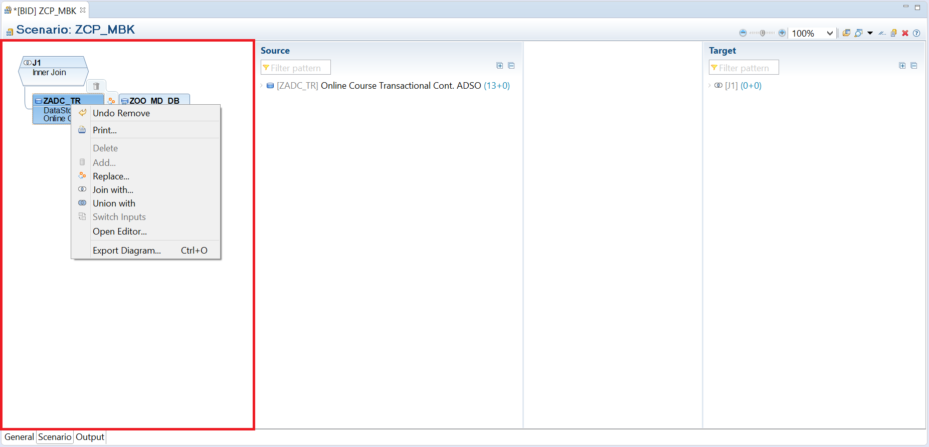
Figure 5. Left side of the Scenario Tab
Furthermore, in the section on the left we can model a Join or a Union. We can model a Join or a Union by either right-clicking the PartProviders or the box indicating the Join or Union itself. After clicking select Join with or Union with (see Figure 6).
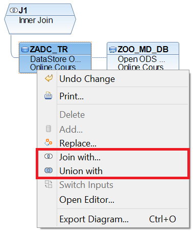
Figure 6. How to Join and Union in the Scenario Tab
In case of a Join, we can choose what kind of join we want (an Inner or Left Outer Join, see Figure 7).
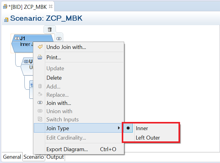
Figure 7. Join Types
I created a test dataset, which I’ll use as an example. The test data is from an imaginary company, “Bailamos” that offers online dancing courses at a fixed price. I’m going to join Bailamos’ transactional data with a master data table containing extra information about the dancing courses. By joining the two table, I can show how a Join in a HCPR works. In our example, we’re going to join an ADSO with transactional data and a Master Data Open ODS View. We’re going to base the Join on the field “Product”.
The “Product” field contains types of online dance courses, such as Salsa and Bachata, that are sold at Bailamos. This “Product” field is present both in our Transactional ADSO and Master Data OODS, which is why we can use it to join the two datasets. All of the values of the “Product” field should be present in both datasets. So we’re going to use an Inner Join, because the result set of an Inner Join only contains records that can be matched in both datasets.
Creating Assignments
In the middle of Figure 8, we see the Source section of the CompositeProvider. We can see the Fact ADSO with Bailamos’ transactional data and the Master Data OODS with additional information about the courses being sold. Once you click a PartProvider on the left side of the Scenario Tab, it shows up in the Source section. It also shows that PartProvider’s fields, if you click the arrow next to the PartProvider in the Source area. On the right, we see the Target area that will contain all the Target fields after we assign the Source fields. The Target fields are the fields that will be available for queries on the HCPR.
We’ve already stated we want to join the transactional dancing data with the master data table on the left. So, now it’s time to assign Source fields to Target fields. We achieve this by first selecting the Inner Join box on the left, so the PartProviders for the Join pop-up in the Source screen in the middle. If you want to add all the fields, right-click a PartProvider in the Source section and click Create Assignments (see Figure 8). In case you only need specific fields, expand the PartProvider tree by clicking on the arrow next to the PartProvider name. Then select the fields you want (i.e. holding CTRL button + clicking), right-click anywhere in the Source area and select Create Assignments.

Figure 8. How to assign your Source fields to a Target field
After assigning your fields you should see some squiggly lines connecting your Source fields to your Target fields, like in Figure 9:
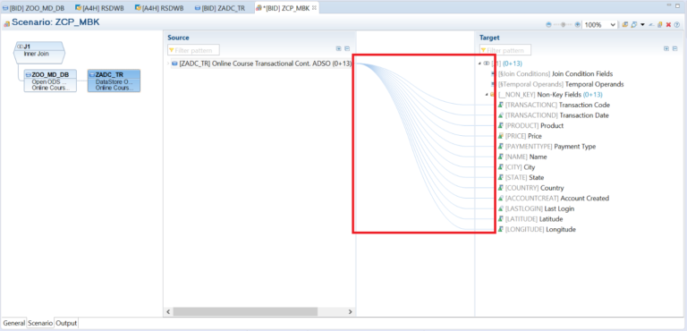
Figure 9. Result of mapping Source fields to your Target
If you do not see all of the fields in your Source provider in the Source area, one of your Source fields probably has a data type that is not compatible with CompositeProviders. How can you see whether that’s the case? Double click your Source InfoProvider and press the ‘Check BW Object’ button (Ctrl+Shift+F2) once you’ve opened your InfoProvider. If you see the message in Figure 10, the field cannot be used in a CompositeProvider:
Figure 10. Field cannot be used in a CompositeProvider
Creating a Join Condition
Now that we’ve mapped our transactional dancing data to the Target, we need to create a Join Condition Field to link it to our Master Data table:
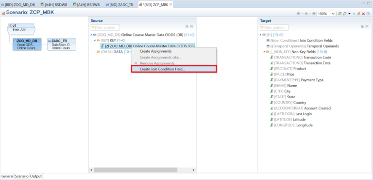
Figure 11. How to create a Join Condition
As we can see in Figure 11, you create a Join Condition Field by right clicking a Source field and pressing the Create Join Condition Field. No Einstein I.Q. needed thus far. After clicking the right option, you end up at the following screen:
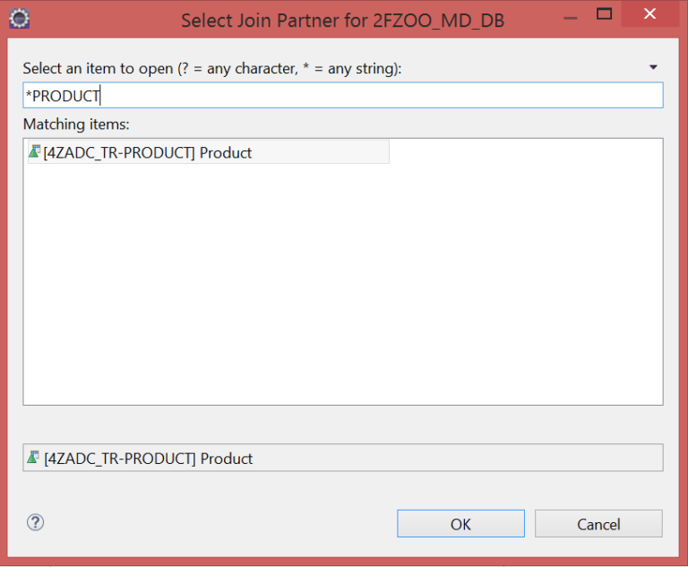
Figure 12. Select Join Partner screen
Next, in Figure 12, we have to select which field to join the field we right-clicked in Figure 11. It’s important you pick a field that has similar values, data type and length, otherwise the Join will backfire. This is especially important when you model an Inner Join (as in our example). Why? Because if an Inner Join does not find any records to match, you’ll end up with a result set of 0 records. We’re going to pick the field “Product”, because it’s uniquely identifies each record in our Master Data and is present in our transactional ADSO. Once you’ve selected the right field to join, you’ll see the Join Condition in the Target area (see following Figure).
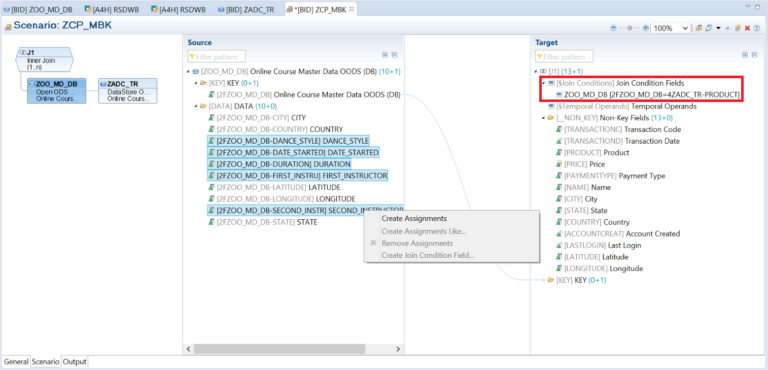
Figure 12a. You can find the Join Condition Fields in the Target area after selecting them
Adding joined fields to the Target
We’re not there yet however, we still need to add the joined fields to our CompositeProvider. To do that, we select the fields we want from our Master Data OODS and click “Create Assignments” (Figure 12a).
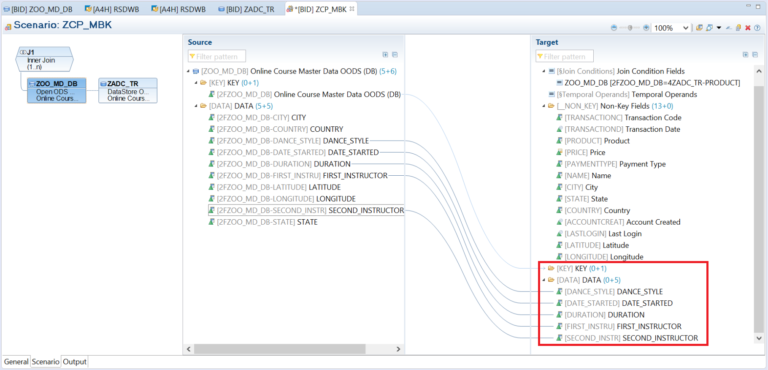
Figure 12b. The result of adding the joined fields to the Target
The result is in Figure 12b. The fields we selected will now be available for querying and our PartProviders will be joined at runtime. How many PartProviders can we join and union? We can create as many joins and unions as we want, but with a few limitations. The first PartProvider you add should be based on transactional data, because you can union the first PartProvider you add as many times as necessary with additional PartProviders. However, you cannot union a PartProvider that you join (see Figure 13). With regards to joins: you can join as many PartProviders you want to the base table, but you cannot perform a join on a join (see Figure 13).
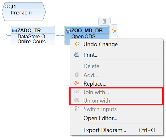
Figure 13. It is not possible to Join or Union a joined PartProvider
Union
In case of a Union, we map similar Source fields to the same field. This mapping is done automatically, when you click Create Assignments (see Figure 14). However, it’s necessary that the fields carry the same data type, length and technical name. We see that the description does not necessarily need to be the same. The Source fields in Figure 8 with a red rectangle have the same technical name “COUNTRY”, but have different descriptions: Country and Land. Because we mapped the Land Source Field first to the Target, the Target field will end up with the description Land, despite being called Country in one of the PartProviders.

Figure 14. Source fields are automatically mapped to the same Target fields with the same data type, length and technical name
The Output Tab
Before we run a query on our CompositeProvider, we’ll have a look at the Output tab from our Inner Join in Figure 15.
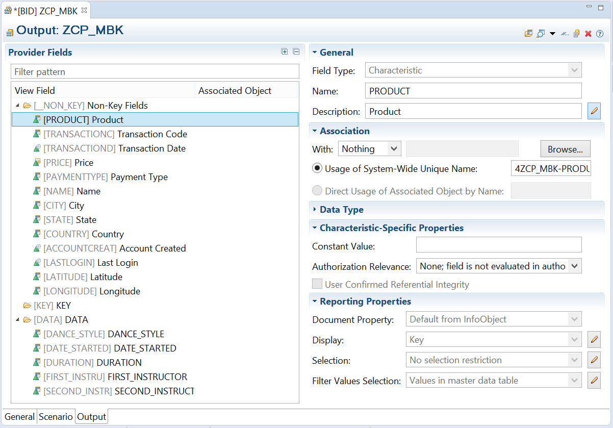
Figure 15. HCPR Output Tab
The Output tab is where you see which fields will be shown in the HCPR. You can also see the properties of those fields in the Output tab. Interestingly, the Output tab is very similar to the Fact/Master Data & Texts tab of the Open ODS View (see Figures 24-26. of Part I of this article). However, HCPR Provider fields in the Output tab are organized in logical groups (such as Key Fields and Non-Key Fields), instead of Data Types (such as Characteristics and Key Figures). To change the logical grouping, press the icon in Figure 16 or right-click any of the maps and select ‘Manage Groups’.
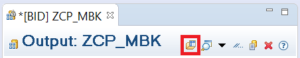
Figure 16. Manage logical grouping
Grouping does not affect query performance, it only exists to organize the fields in a logical way.
Performing a Query
BW Reporting Preview
Now that we’ve seen all the different tabs, let’s perform a Data Preview on our newly modeled CompositeProvider. To perform a Data Preview, press the button in Figure 17.

Figure 17. How to access the BW Reporting Previewer
We can see what the output looks like in Figure 18.
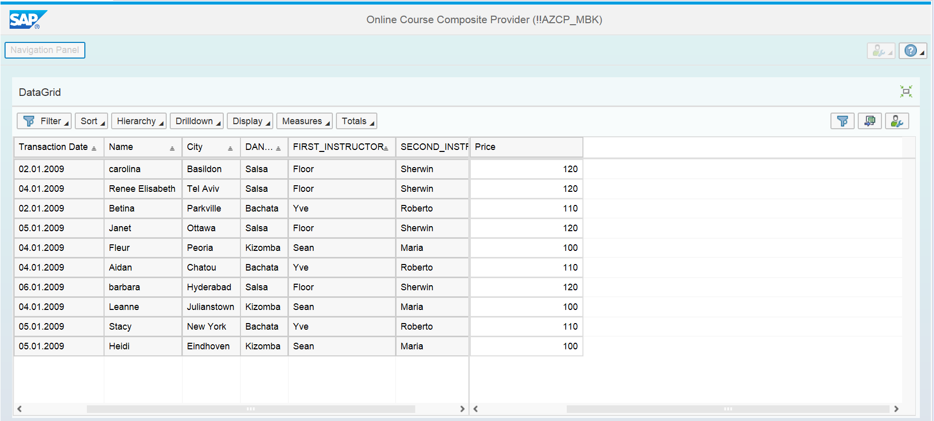
Figure 18. Query result of Data Preview in Eclipse
The modeling of our CompositeProvider was a success! How can we tell? Well first of all: if our Inner Join hadn’t worked, we would have had a result set of 0 records in Figure 18. Secondly, in the fifth and sixth column of Figure 18, we see the field values of all the Dancing Course Instructors. We would not have known that Yve was Betina’s dance instructor if the Join had not worked. Originally, the underlying ADSO contained the information about which customers ordered what, and our Open ODS View Master Data table contained the info about instructors.
As a final check, we’re going to compare the sum of the measures in the HCPR to the sum of the measures in our Fact ADSO. That way we can determine whether our join is duplicating any data due to a n:m relation. The sum of the measures in the HCPR is equal to the sum of the measures in the fact table (1.110), so our Join is not duplicating any data.
BusinessObjects Analysis
Mission Complete! However, if you’re like me you still won’t be happy. My source of unhappiness? The unintuitive BW Reporting Previewer that is available in Eclipse. For instance, if you select 10 characteristics it may initially only show about 4. Also, it does not let you edit the amount of space designated to measures (even if you only have 1). That is why I would recommend, to execute a query on your CompositeProvider by using SAP BusinessObjects Analysis (see Figure 19).
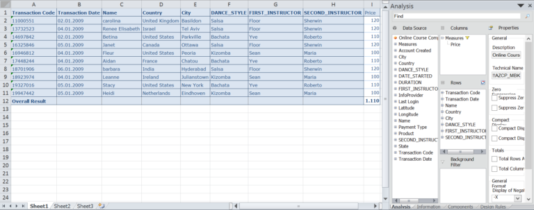
Figure 19. Running a query from BO Analysis
Once I queried the CompositeProvider in Analysis I let out a sigh of relief. My forehead also instantaneously got less warm from the reduced stress of not having to try and query InfoProviders with the Eclipse BW Reporting Previewer. The result in Excel is nice and clear, we instantly have a nice overview of the fields we want to see. Also, in Analysis we’re able to quickly access navigational attributes and texts by clicking on the plus sign.
In Figure 19, we also see fields from the Master Data Open ODS View as well as fields from the Transactional ADSO. In row 8 we can see that Sherwin is the second instructor (Master Data) of Barbara from India (Transactional Data). We can also see Barbara’s Transaction Code and the price she paid (Transactional Data) to be able to dance Salsa (Master Data). The world of online dancing courses has just become more transparent!
Association
I used the a Transactional ADSO and Master Data OODS as an example to demonstrate how to perform a Join and Union in a CompositeProvider. However, the standard way to include a Master Data OODS or Text OODS in a HCPR is via association. By associating a Characteristic field in a HCPR to an InfoObject or Open ODS View, the HCPR Characteristic field inherits the Navigational Attributes and Texts of the associated InfoObject or Open ODS View. I’ll give you an example of how to do it:
Because we’re going to add the Master Data OODS fields via Association, we only need to include the transactional ADSO in the Scenario Tab (see Figure 20).
Figure 20. No need to add a Master Data OODS in the Scenario Tab when using Association
After modeling our transactional ADSO, we need to associate one of our HCPR Output fields with our Master Data OODS. In the Output screen of the CompositeProvider, we go to the Association section on the right and select Open ODS (see Figure 21). Then we select the Master Data OODS that we created in Figure 25 of Part I of this article. After Association, the Master Data OODS will appear in the Provider Fields section on the left of the Output tab. The field we are associating here, Product, has the same data type, length and values as the Representative Key Field in the Master Data OODS. Because of that BW will successfully join the Product field in our CompositeProvider with the one in the Master Data OODS during runtime.
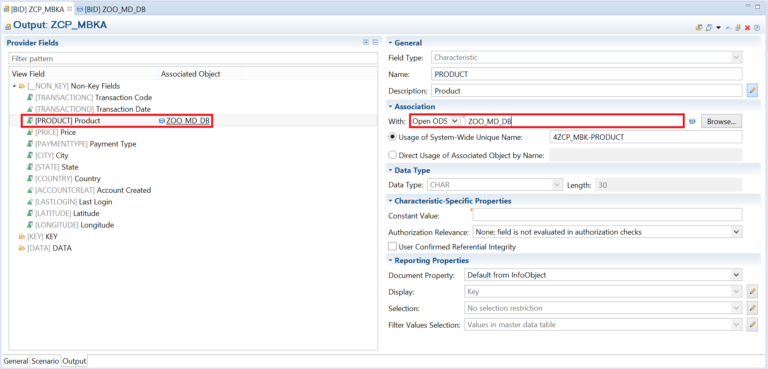
Figure 21. Associating a CompositeProvider field with an OODS to use Navigational Attributes
Because we associated the Master Data OODS with the Product field, we are now able to use the fields in the Master Data OODS as Navigational Attributes (see Figure 19). Just like in Figure 19, we can see that Sherwin is Barbara’s second instructor:
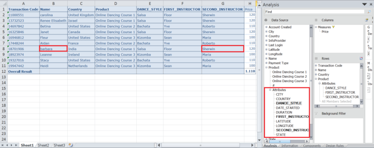
Figure 22. Using Master Data OODS fields as Attributes in queries on CompositeProviders
Association works if you can join transactional data with a Master Data OODS based on one field. However, for more complicated joins it’s better to either use a HCPR join or use custom logic in a Transformation.
Pros & cons
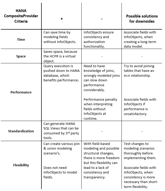
Table 1. HANA CompositeProvider criteria
Finally, here’s an overview of the pros and cons of the HANA CompositeProvider:
Virtual Sanity
Together with Part I of this article, you are now equipped with the knowledge necessary to go virtual in BW! In Part II of this article, we’ve learned why we need a HANA CompositeProvider. We now also know how to model CompositeProviders. We’ve learned how to select a Union or Join type, how to assign Source fields to Target fields and how to use Association. Hopefully, you can now avoid (virtual) insanity by executing queries in BO Analysis instead of the BW Reporting Previewer. Jamiroquai would be proud of you!
This article belongs to
Tags
- BW
- BW4HANA
- Composite Provider
- CompositeProvider
- Eclipse
- HANA
- HCPR
- Virtual
Author
- Michael Bussink